Turning Robot Motion into Fluid Art
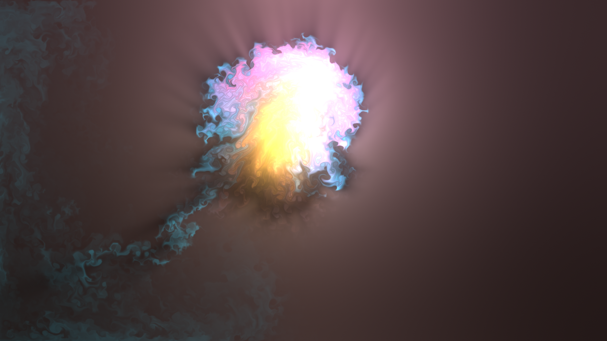 Demo
Demo I found a 2D WebGL fluid simulation on GitHub’s trending page one Friday afternoon and lost about twenty minutes clicking around the canvas watching colors swirl. I forgot what I was actually doing. Then I started thinking about how it would look as a ROS node.
You map the arm’s end-effector motion to perturbations in the fluid field. X and Y position control where on the screen the perturbation appears, Z controls the radius, and the orientation of the end-effector (as a quaternion) maps to the color. Move the arm around and you get trails of color flowing across the screen in real time. It looks way cooler than it has any right to. I built the whole thing over a weekend.
The Core Idea
You have a simulated UR3e robot arm playing back pre-recorded paths, and a WebGL fluid simulation running in a browser. A ROS node sits in between, listening to the TF transform tree for the end-effector’s pose and translating that into visualization events.
The coordinate mapping works like this:
- X, Y Positions map directly to screen offsets from center. The robot’s workspace gets normalized to [-1, 1] range across the canvas.
- Z Position controls the perturbation radius. Higher Z means a bigger splat. The formula is simple: normalize Z into [0, 1] and feed it to the simulator as the radius parameter.
- Orientation maps to color through Euler angles. Roll goes to the red channel, pitch to green, yaw to blue. Each angle gets normalized from [-pi, pi] into a color intensity. So as the end-effector rotates through a path, the fluid trails shift in hue.
The result is that every path the robot traces gets rendered as its own fluid signature. It’s an intuitive way to see what a robot arm is doing spatially.
Architecture
The system is split between a ROS backend and a web frontend, connected through ROS Bridge (WebSocket on port 9090).
On the ROS side, a trajectory_visualizer node does the heavy lifting. It polls the TF tree for the end-effector’s pose relative to base_link, computes the screen coordinates and color mapping, then publishes trajectory events (start, update, stop) as the arm moves. There are also ROS services for updating the visualization config (color overrides, radius adjustments) on the fly.
On the browser side, a small script (ros-node.js) subscribes to those trajectory topics and translates them into calls against the fluid simulator’s API. The simulator itself is a modified version of PavelDoGreat’s original code with a few hooks added for external control: visualize_trajectoryStart(), visualize_trajectoryUpdate(), visualize_trajectoryStop(), and config getter/setters. The fluid engine is doing real incompressible fluid dynamics in WebGL shaders (pressure projection, vorticity confinement, advection, the works) so the swirls come from a real flow solve, not a canned particle effect.
The nice thing about the ROS Bridge approach is that the visualization is completely decoupled from the robot stack. Any browser on the network can open localhost:8080 and see the fluid sim. You could theoretically point it at a real robot’s TF tree instead of a simulated one and it would just work.
Three Planners, Three Personalities
I integrated support for three different motion planners, partly because I had them available from my Motion Playground project on the same UR3e platform (that project grew up alongside this one and has its own post), and partly because it was interesting to see how each planner’s behavior shows up visually in the fluid.
OMPL (via MoveIt) is the default sampling-based planner. It generates waypoint-to-waypoint trajectories through joint space, so the end-effector paths tend to be indirect. In the fluid visualization, OMPL paths produce these arcing, sometimes jerky streams. You can really see the planner “thinking” as it navigates around joint limits.
RelaxedIK is a real-time IK solver out of UW’s Graphics group that handles singularities and self-collision avoidance gracefully. Since it’s solving continuously rather than planning discrete trajectories, the paths come out much smoother, and its traces render as clean, flowing lines. The difference from OMPL is immediately obvious just watching the colors move.
LivelyIK is a fork of RelaxedIK from the Wisc-HCI group that adds Perlin noise to the solver, making the robot’s motion appear more lifelike. In the fluid visualization, this shows up as a subtle organic wobble in the trails. Where RelaxedIK draws clean lines, LivelyIK draws lines that breathe a little. It’s a small difference but a visually interesting one.
For RelaxedIK and LivelyIK, I wrote a path reader that does linear interpolation between waypoints (with SLERP for the orientations) to give the solvers something smooth to track. There’s also a configurable hold at each waypoint to let the solver catch up before moving on. The MoveIt path reader is simpler since MoveIt handles its own interpolation internally.
Path Recording
I included a small terminal utility (path_saver.py) for recording custom paths. You launch it alongside RViz, drag the robot’s end-effector to where you want it, press Enter to save the pose, repeat, and then press q when you’re done. It dumps the waypoints to a JSON file that any of the three path readers can pick up.
The JSON format is minimal: a list of poses (position as [x, y, z], orientation as a quaternion [x, y, z, w]) plus metadata about the reference frames. Nothing fancy, but it means you can hand-author paths too if you want to get specific about the geometry.
Lessons Learned
The fluid sim is sensitive to path quality. Smooth, continuous motion produces beautiful results. Jerky, discontinuous motion (like what you sometimes get from OMPL’s sampling) produces visual noise. The visualization inadvertently became a quality metric for planner output.
Mapping orientation to color is more informative than I expected. I added it mostly because I had the data available and wanted to use it for something. But it turns out that watching the color shift as the arm rotates through a path gives you real spatial intuition about what the end-effector is doing. Constant color means the orientation is stable. Rapid hue changes mean the arm is reorienting aggressively. It’s the kind of thing that’s hard to see in RViz but obvious in the fluid sim.
WebGL fluid simulation is just fun to watch. Even after the novelty of the robotics integration wore off, I’d catch myself leaving the browser tab open and watching the patterns develop. There’s something meditative about it. The bloom and sunray post-processing effects in the shader definitely contribute to that.
Conclusion
I built this because I saw a cool fluid sim and wanted to know what it would look like driven by a robot arm. It looks pretty great, and that was reason enough for a weekend.
It also turned out a little more useful than I planned. There might be a real trajectory sanity check in the swirls, or just another window to leave open while a robot works. I never pushed it that far. If I come back to it, the first thing I would do is point it at a real arm’s TF tree instead of the simulated one. The ROS Bridge split means that should only be a config change. I have not tried it.
Check out the GitHub Repository.
Thanks for reading. Stay tuned and keep building.